XPS for Beginners
- XPS Course Fundamentals
- XPS Data Analysis
Welcome to the data analysis section of our XPS for Beginners course!
We start in part 4, with a look at the basics of fitting peaks in XPS.
Open the dataset by downloading from the link above and opening in CasaXPS
Try and model the data using component fitting as described in the above tutorial.
Sections below will describe a detailed process for each sample
- PTFE
- PET
- PVP
- Oxalic acid
PTFE is a very simple polymer for us to start with – one carbon environment and one fluorine environment. This is just a chance to put in some components and make sure you are comfortable with the process.

PET has 3 carbon environments in a ratio of 6:2:2

So if we fit 3 components we can look at the area ratios (and % ratios) to determine we have the correct amounts of each carbon environment.

You may note we have fit our region around a small shoulder at around 288 eV. This is a shake up feature from the π-π* MO in the aromatic ring and we need to include it in our background to properly fit the peaks!
Note the % concentration in the very bottom row of the quantification window. Our carbon % are roughly in-line with our expectations, though with a little more CC than expected. This is likely due to adventitious carbon and would be reduced were we to clean the surface using argon ion clusters.
PVP has 3 CC/CH environments, 2 C-N environments, and 1 N(C=O)C environment.

Again, we can use the ‘Area constraint’ function to help us model this compound – since we know the ratios to expect.
Locking to peak C (the carbonyl) will be simplest, since it is a single carbon, allowing us to lock the CC/CH peak area to ‘C*3’ and the C-N peak to ‘C*2’. Again, FWHM are locked to be equivalent.

N and O peaks represent a single environment, and can be fit as a single peak.
First apply a region to the C 1s spectra
Notice that we are expecting a single carbon peak – but in reality here we see 2 carbon peaks.

This is due to adsorbed adventitious carbon, which we can actually use for charge referencing.

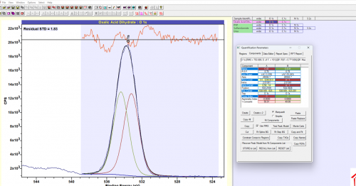
Fitting the C 1s region with 3 peaks allows us to distinguish the oxalic carbons vs the adventitious carbons. Note we are using ‘A*1’ in the FWHM constraint box of columns B and C to ensure the peak widths all remain constant.
For O 1s, we are actually constraining both the FWHM and peak area of the 2 oxygens. In reality there is likely some contribution from oxygen containing adventitious carbon, which is making our fit a little worse than expected.
