XPS for Beginners
- XPS Course Fundamentals
- Data Analysis
- Applications of XPS
- Related Techniques
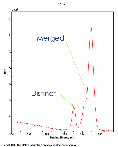
XPS spectra do not only contain clear, distinct peaks for each chemical environment
More often than not, the energy separation is not large enough to divide the emissions into individual peaks
This means, while we might get some clear peaks, many will merge into a single envelope
This means we need a method by which to model the individual components that make up a peak envelope
We have mentioned in a previous section, that the peaks in XPS tend to be a convolution of a Gaussian form (instrumental broadening) and Lorentzian form (intrinsic broadening)
We can use a model lineshape based on this theory to probe our data
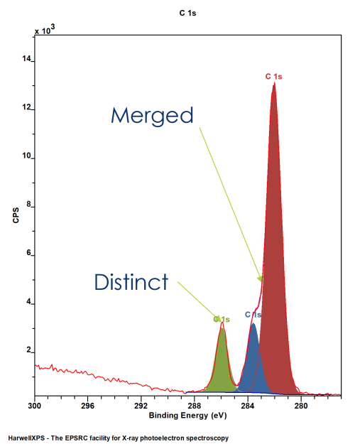
Historically used for peak fitting, less advised in recent years but will be commonly found in literature
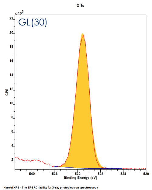
Convolution of G:L in a ratio defined by the function – GL(X) (0 < X < 100)
GL(100) = Lorentzian, GL(0) = Gaussian
GL(30) commonly used lineshape
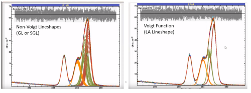
Voigt-type function
LA lineshapes generally recommended for fitting symmetric peaks
Better reflect real peak shapes
Form LA(a, m) – a = tail spread, m = width of Gaussian modifier

LA lineshapes may be modified to account for peak asymmetry
LA(a, β, m) – now a & β modify the tail spread at high and low binding energy independently
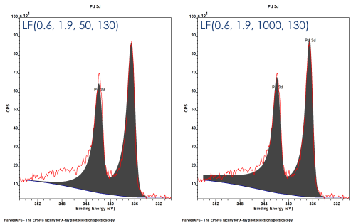
LF form is the same as the LA form but with an additional modifier
LF(a, β, w, m) – where w = damping modifier (1 < w < 1000)
Not necessarily physically accurate – but can help produce good models within confines of data range
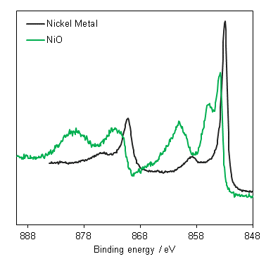
Peak modelling is a powerful tool for understanding XPS spectra – but it is not always necessary!!
In many cases, XPS can be used to either confirm properties based on literature studies (e.g. Binding energies of pure materials) or as a fingerprint technique (e.g. complicated first row TM spectra).
Fitting can be time consuming and often introduce errors if not performed properly
Biggest mistake in published peer reviewed data!
